Hermite插值多项式
Hermite插值是一种插值方法,可以通过给定的点和导数值构造插值多项式。给定点\((x_0,y_0),(x_1,y_1),...,(x_n,y_n)\) 和导数值\(y'_0,y'_1,...,y'_n\) ,可以构造插值多项式。本文介绍如何使用Newton差商生成Hermite插值多项式。
Newton差商
Newton差商公式是一个递归定义的公式,可以写成一个表格的形式:
\[
f[x_i,x_{i+1},...,x_{i+j}]=\frac{f[x_{i+1},x_{i+2},...,x_{i+j}]-f[x_i,x_{i+1},...,x_{i+j-1}]}{x_{i+j}-x_i}\tag{1}
\]
给定一组点\((x_0,y_0),(x_1,y_1),...,(x_n,y_n)\) ,可以通过差商表格计算出插值多项式的系数。第一列和第二列分别是\(x_i\) 和\(y_i\) ,后面的列是差商,通过递归公式一列一列地计算出来。下面是一个生成差商表格的Python函数:
1
2
3
4
5
6
7
8
9
10
11
12
13
14
15
16
17
18
19
20
21
import numpy as npimport matplotlib.pyplot as pltimport pandas as pdimport sympy as spdef generate_newton_diff_quotient_table (x, y ): max_order = len (x) - 1 newton_diff_quotient_table = pd.DataFrame(np.zeros((len (x), max_order + 2 ))) for i in range (len (x)): newton_diff_quotient_table.iloc[i, 0 ] = x[i] newton_diff_quotient_table.iloc[i, 1 ] = y[i] for i in range (0 , len (newton_diff_quotient_table.columns) - 2 ): for j in range (i + 1 , len (newton_diff_quotient_table)): newton_diff_quotient_table.iloc[j, i + 2 ] = ( newton_diff_quotient_table.iloc[j, i + 1 ] - newton_diff_quotient_table.iloc[j - 1 , i + 1 ] ) / ( newton_diff_quotient_table.iloc[j, 0 ] - newton_diff_quotient_table.iloc[j - i - 1 , 0 ] ) return newton_diff_quotient_table
比如给定点\((0,0),(1,16),(2,46),(3,94),(4,160)\) ,可以生成差商表格:
1
2
3
4
x = [0 , 1 , 2 , 3 , 4 ] y = [0 , 16 , 46 , 94 , 160 ] newton_diff_quotient_table = generate_newton_diff_quotient_table(x, y) print (newton_diff_quotient_table)
输出结果:
\(x\) \(y\) \(f[x_0,x_1]\) \(f[x_0,x_1,x_2]\) \(f[x_0,x_1,x_2,x_3]\) \(f[x_0,x_1,x_2,x_3,x_4]\)
0
0
0
0
0
0
1
16
16
0
0
0
2
46
30
7
0
0
3
94
48
9
0.666667
0
4
160
66
9
0
-0.166667
Newton插值
用Newton差商可以得到插值多项式的系数,然后可以用这些系数构造插值多项式。插值多项式的形式是:
\[
p(x)=f[x_0]+\sum_{i=1}^{n}f[x_0,x_1,...,x_i]\prod_{j=0}^{i-1}(x-x_j)\tag{2}
\]
用上一节生成的差商表格,可以写出
\[
p(x)=(x-0)+16(x-0)(x-1)+7(x-0)(x-1)(x-2)+\frac{2}{3}(x-0)(x-1)(x-2)(x-3)\tag{3}
\] 可以看出,插值多项式的系数是差商表格的对角线元素。
1
2
3
4
5
6
7
8
9
10
def newton_interpolation (tb ): x = sp.symbols("x" ) n = len (tb.columns) - 2 p = tb.iloc[0 , 1 ] for i in range (1 , n + 1 ): term = tb.iloc[i, i + 1 ] for j in range (0 , i): term *= x - tb.iloc[j, 0 ] p += term return p
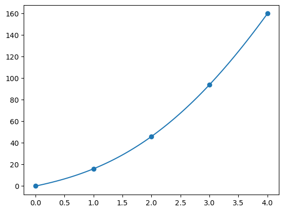
绘制插值多项式:
1
2
3
4
5
6
7
8
def plot_interpolation (p, x, y ): xx = np.linspace(x[0 ], x[-1 ], 100 ) plt.plot(xx, [p.subs("x" , i) for i in xx]) plt.scatter(x, y) plt.show() p = newton_interpolation(newton_diff_quotient_table) plot_interpolation(p, x, y)
Hermite插值
在Newton差商表格的基础上,重复每个点两次,并且设置其导数值作为一阶差商。然后使用原来的计算方法生成差商表格,跳过已经计算过的差商(已知的导数),使用和Newton插值多项式一样的方法就可以得到Hermite插值多项式。
下面是一个用于生成Hermite插值多项式的生成Newton差商表格的Python函数:
1
2
3
4
5
6
7
8
9
10
11
12
13
14
15
16
17
18
19
20
21
def generate_hermite_diff_quotient_table (x, y, y_prime ): max_order = len (x) * 2 - 1 newton_diff_quotient_table = pd.DataFrame(np.zeros((len (x) * 2 , max_order + 2 ))) newton_diff_quotient_table.iloc[:, :] = 999999 for i in range (len (x)): newton_diff_quotient_table.iloc[i * 2 , 0 ] = x[i] newton_diff_quotient_table.iloc[i * 2 + 1 , 0 ] = x[i] newton_diff_quotient_table.iloc[i * 2 , 1 ] = y[i] newton_diff_quotient_table.iloc[i * 2 + 1 , 1 ] = y[i] newton_diff_quotient_table.iloc[i * 2 + 1 , 2 ] = y_prime[i] for i in range (0 , len (newton_diff_quotient_table.columns) - 2 ): for j in range (i + 1 , len (newton_diff_quotient_table)): if newton_diff_quotient_table.iloc[j, i + 2 ] == 999999 : newton_diff_quotient_table.iloc[j, i + 2 ] = ( newton_diff_quotient_table.iloc[j, i + 1 ] - newton_diff_quotient_table.iloc[j - 1 , i + 1 ] ) / ( newton_diff_quotient_table.iloc[j, 0 ] - newton_diff_quotient_table.iloc[j - i - 1 , 0 ] ) return newton_diff_quotient_table
比如给定点\((0,0),(1,16),(2,46),(3,94),(4,160)\) 和导数值\(0.5,0.8,1.2,1.8\) ,可以生成差商表格:
1
2
3
4
5
x = [0 , 1 , 2 , 3 , 4 ] y = [0 , 16 , 46 , 94 , 160 ] y_prime = [0.5 , 0.5 , 0.8 , 1.2 , 1.8 ] hermite_diff_quotient_table = generate_hermite_diff_quotient_table(x, y, y_prime) print (hermite_diff_quotient_table)
\(x\) \(y\) \(f[x_0,x_0]\) \(f[x_0,x_0,x_1]\) \(f[x_0,x_0,x_1,x_1]\) \(f[x_0,x_0,x_1,x_1,x_2]\) \(f[x_0,x_0,x_1,x_1,x_2,x_2]\) \(f[x_0,x_0,x_1,x_1,x_2,x_2,x_3]\) \(f[x_0,x_0,x_1,x_1,x_2,x_2,x_3,x_3]\) \(f[x_0,x_0,x_1,x_1,x_2,x_2,x_3,x_3,x_4]\) \(f[x_0,x_0,x_1,x_1,x_2,x_2,x_3,x_3,x_4,x_4]\)
0.0
0.0
/
/
/
/
/
/
/
/
/
0.0
0.0
0.5
/
/
/
/
/
/
/
/
1.0
16.0
16.0
15.5
/
/
/
/
/
/
/
1.0
16.0
0.5
-15.5
-31.0
/
/
/
/
/
/
2.0
46.0
30.0
29.5
22.5
26.75
/
/
/
/
/
2.0
46.0
0.8
-29.2
-58.7
-40.60
-33.675000
/
/
/
/
3.0
94.0
48.0
47.2
38.2
48.45
29.683333
21.119444
/
/
/
3.0
94.0
1.2
-46.8
-94.0
-66.10
-57.275000
-28.986111
-16.701852
/
/
4.0
160.0
66.0
64.8
55.8
74.90
47.000000
34.758333
15.936111
8.159491
/
4.0
160.0
1.8
-64.2
-129.0
-92.40
-83.650000
-43.550000
-26.102778
-10.509722
-4.667303
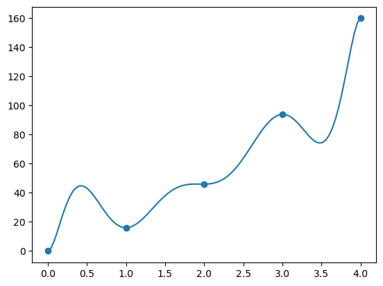
然后可以用和Newton插值多项式一样的方法生成Hermite插值多项式:
\[
p(x)=0+0.5(x-0)+15.5(x-0)(x-0)+-31(x-0)(x-0)(x-1)+26.75(x-0)(x-0)(x-1)(x-1)+-33.675(x-0)(x-0)(x-1)(x-1)(x-2)+21.119444(x-0)(x-0)(x-1)(x-1)(x-2)(x-2)+-16.701852(x-0)(x-0)(x-1)(x-1)(x-2)(x-2)(x-3)+8.159491(x-0)(x-0)(x-1)(x-1)(x-2)(x-2)(x-3)(x-3)-4.667303(x-0)(x-0)(x-1)(x-1)(x-2)(x-2)(x-3)(x-3)(x-4)
\]
1
2
p = newton_interpolation(hermite_diff_quotient_table) plot_interpolation(p, x, y)
测试该插值多项式在给定点的导数值:
1
2
3
4
5
6
7
8
9
10
11
12
13
14
15
16
17
18
19
20
21
22
23
def test_interpolation (p, x, y, y_prime=None ): if ( abs (p.subs("x" , x) - y) < 1e-10 and (y_prime is None or abs (p.diff("x" ).subs("x" , x) - y_prime) < 1e-10 ) ): return True else : print ("p.subs('x',x) = {0}, y = {1}" .format (p.subs("x" , x), y)) if y_prime is not None : print ( "p.diff('x').subs('x',x) = {0}, y_prime = {1}" .format ( p.diff("x" ).subs("x" , x), y_prime ) ) return False def test_interpolations (p, x, y, y_prime=None ): for i in range (len (x)): if not test_interpolation(p, x[i], y[i], y_prime[i] if y_prime is not None else None ): return False return True test_interpolations(p, x, y, dydx)
返回True,说明插值多项式在给定点的导数值是正确的。